
If a computer captions a photo in the forest, and no one reads it, did it really see anything?
Today, models can understand visual context in images and generate captions almost like a human. But it all started with simple CNN+LSTM models, which barely understood what was in an image. I decided to explore how a computer can “see” and describe the world around it. In this article, I’ll show you how to implement and train three models from scratch: Show & Tell, Show Attend and Tell, and a ViT+Transformer decoder. You’ll see the evolution of image captioning approaches and be able to try it yourself at home.
You can also find the complete code for all models here.
Why We Want Computers to Write Poems About Your Pictures
Image captioning is the task of generating a textual description of an image. It is used in:
- Automatic photo captions (Instagram, Flickr).
- Assistive technologies for visually impaired people.
- Autonomous cars and robots that need to understand their surroundings.
A brief evolution of models:
- Show & Tell (2015) — CNN → LSTM.
- Show Attend and Tell (2016) — added attention so the model could focus on objects.
- ViT + Transformer (2020+) — modern transformers that understand the full visual context.
- Multimodal Transformers / CLIP + GPT (2021+) — models that combine vision and language, enabling understanding and generation across both modalities.
Dataset and Evaluation
All models were trained and evaluated using the MS COCO image captioning dataset.
| Model | Training Data | Validation Data |
|---|---|---|
| Show & Tell | COCO train2014 + train2017 | COCO val2017 |
| Show Attend and Tell | COCO train2014 + train2017 | COCO val2017 |
| ViT + Transformer Decoder | COCO train2017 | COCO val2017 |
Model performance was evaluated using two standard image captioning metrics:
BLEU-4 measures how closely a generated caption matches reference captions by comparing word sequences (n-grams) of lengths 1 to 4. For example, in "A black cat sits on the sofa", it evaluates individual words (cat), word pairs (black cat), triples (a black cat), and four-word sequences (a black cat sits). The metric combines the precision of these matches and penalizes overly short captions.
CIDEr also compares n-grams of lengths 1 to 4, but uses TF-IDF weighting to emphasize informative word sequences. Common expressions such as "the" or "on" receive lower weights, while more distinctive phrases such as "black cat" may receive higher weights. Unlike BLEU-4, CIDEr measures similarity using weighted n-gram vectors and is designed to reward agreement with multiple human-written captions.
The classic that explains it all: Show & Tell
Let’s dive straight into how these architectures work, moving from the simple to the more complex.
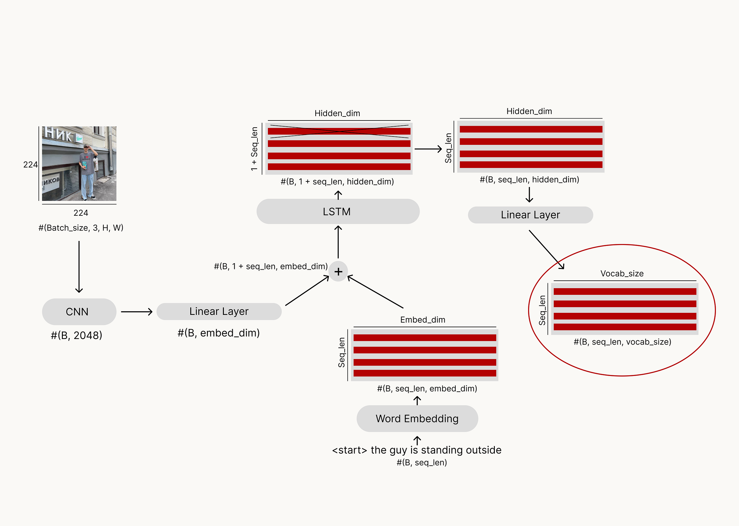
Main idea: Architecture: CNN encoder + LSTM decoder.
Key steps:
- The CNN extracts features from the image.
- The LSTM generates a sequence of words.
Training: During training, the logic works as follows: ResNet50 extracts the visual context, and the LSTM is fed the correct sentence right away — but with a start token at the beginning to begin prediction. We only consider predictions after the first token (the start token), because it signals to the model that sentence generation has started. The predictions are then compared with the target sentence, whose last word is the end token. The model receives the correct sentence immediately to help it converge properly — this approach is called teacher forcing.
Prediction: During inference, the model receives the image and the start token. After that, it feeds its own previous predictions back as input at each step. This process continues until the model predicts the end token, generating the full caption.
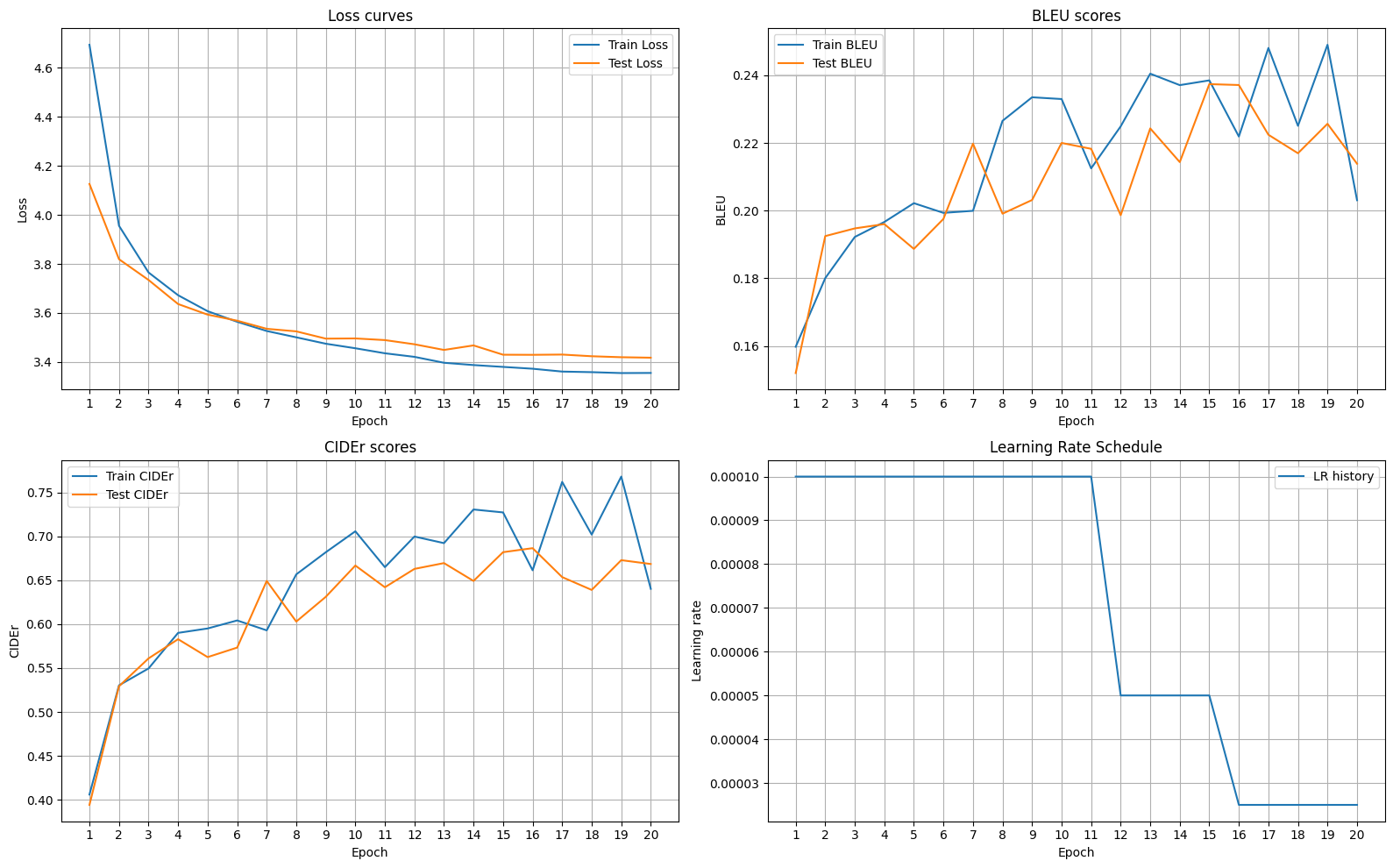
I trained the model with the following parameters:
- embed_size = 512 — the size of the word embeddings fed into the LSTM.
- hidden_size = 512 — the size of the LSTM’s hidden state.
- num_layers = 1 — a single-layer LSTM.
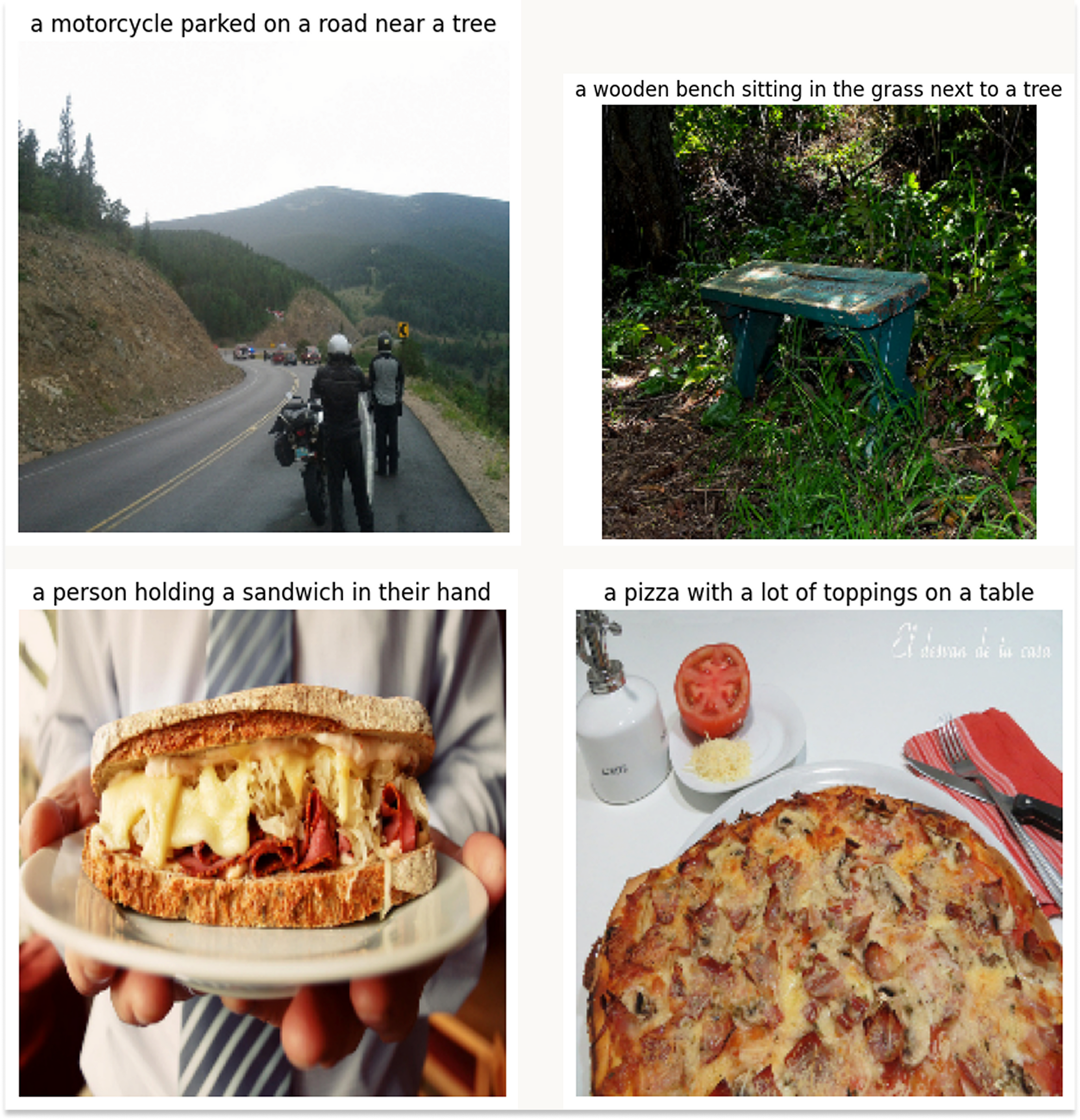
Let’s take a look at some examples of captions generated by the model:
We obtain the following metrics:
| Decoding Strategy | BLEU-4 Score | CIDEr Score |
|---|---|---|
| Greedy | 0.20 | 0.62 |
| Beam Search | 0.198 | 0.616 |
Pros
- Simple and understandable architecture: a separate CNN for the image and an LSTM for the text.
- Easy to train and converges quickly on small datasets.
- Great for educational purposes and initial experiments in caption generation.
Cons
- Sees the image as a single feature vector → loses local information.
- Cannot focus on important objects, so captions may be generic or miss details.
- Sensitive to sentence length and image complexity.
- During generation without teacher forcing, errors accumulate because the model relies on its own predictions.
Tip: You can try this implementation yourself — full code is available here.
Greedy and Beam Search strategy
Let’s take a short detour and understand how the greedy strategy differs from beam search.
Greedy decoding: at each step, the model simply picks the most probable word. It’s fast and simple but can easily miss the best overall caption — a locally optimal choice may lead to a worse global result.
Beam search: the model takes the top K words with the highest scores, then for each of those words, it again takes the top K next words — forming a tree of possible sentences. At the end, it selects the sentence with the highest total sum of log probabilities, which represents the most likely overall caption according to the model.
Attention: Show Attend and Tell
How do people describe a photo? First, we notice the main object, then we talk about the background, and finally we start noticing smaller details — this is how we create a complete description of what’s happening in the image. The same idea was applied to models: they were given attention mechanisms.
Our next architecture, Show Attend and Tell, does everything the previous model did, but before generating the next word, it looks at the image again through the lens of the words it has already generated.
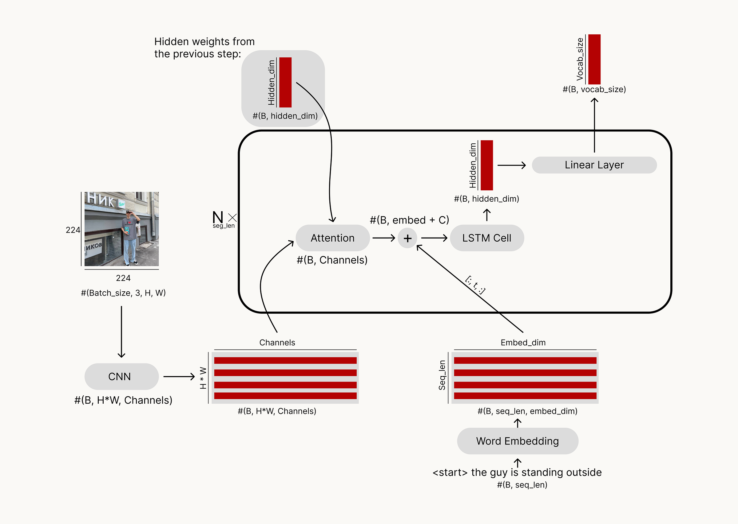
Main idea: Architecture: CNN encoder + LSTM decoder, but with an attention mechanism between them.
Key steps:
- The CNN extracts features from the image.
- The model determines where to focus in the image for generating the next word.
- The LSTM generates the sequence of words, using both the visual features and the attention context.
Training: During training, the logic works as follows: ResNet101 extracts the visual context, which is then used to initialize the hidden states of the LSTM. Using attention, the model looks at the visual context through the lens of the LSTM’s hidden states and computes attention weights. These attention weights are combined with the word embeddings and passed through the LSTM. As in the previous model, during training we feed the entire correct sentence and compare the outputs to the target.
Tip: Here, I also applied a trick called scheduled sampling: with a certain probability, the model receives its own previous prediction instead of the correct word. This helps the model learn to recover from its own mistakes and improves robustness during inference.
Prediction: Everything works like during training, but the model feeds its own previous prediction as input to generate the next word.
I trained the model with the following parameters:
- embed_size = 512 — the size of the word embeddings fed into the LSTM.
- hidden_size = 512 — the size of the LSTM’s hidden state.
- num_layers = 1 — a single-layer LSTM.
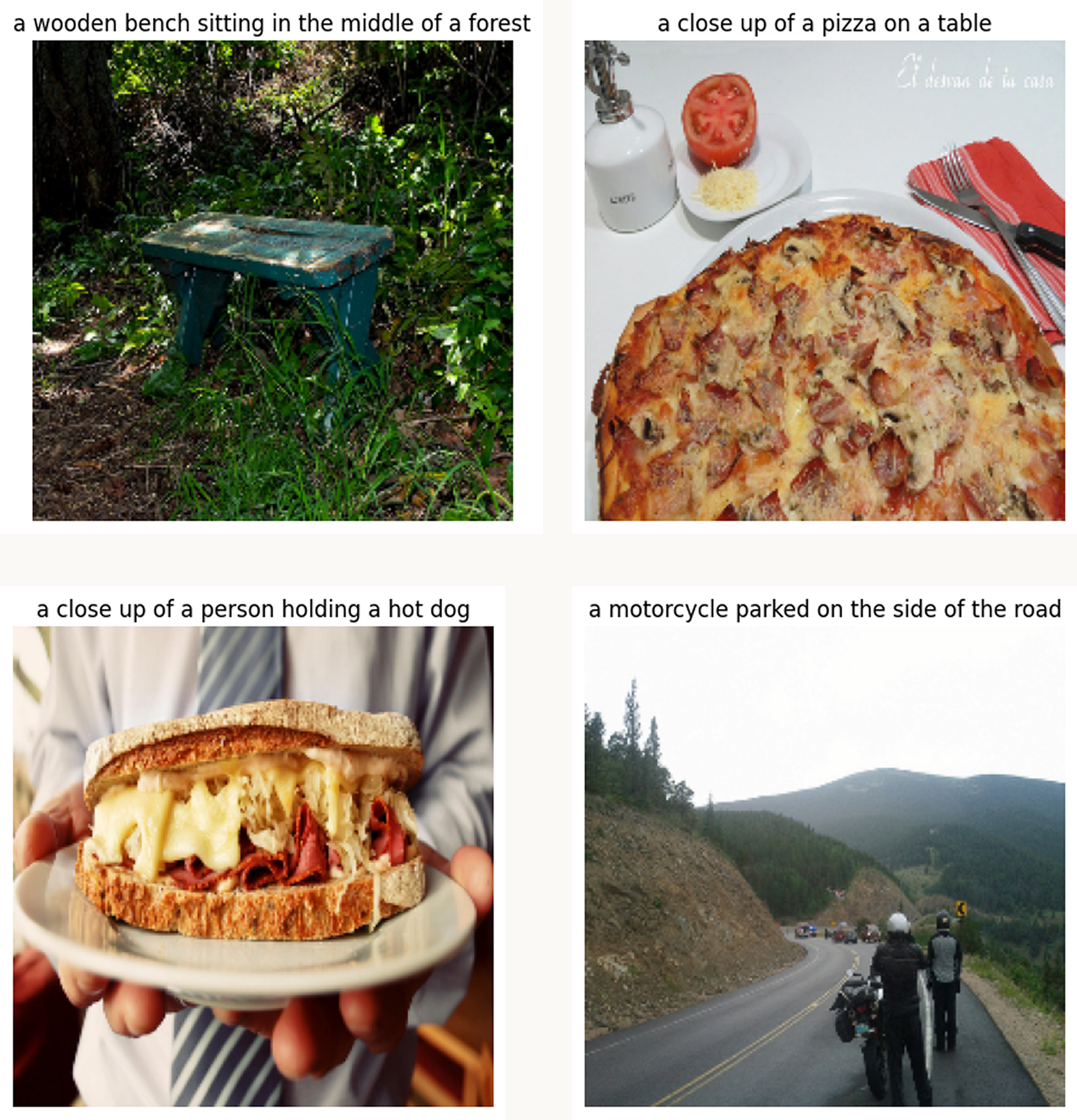
Let’s take a look at some examples of captions generated by the model:
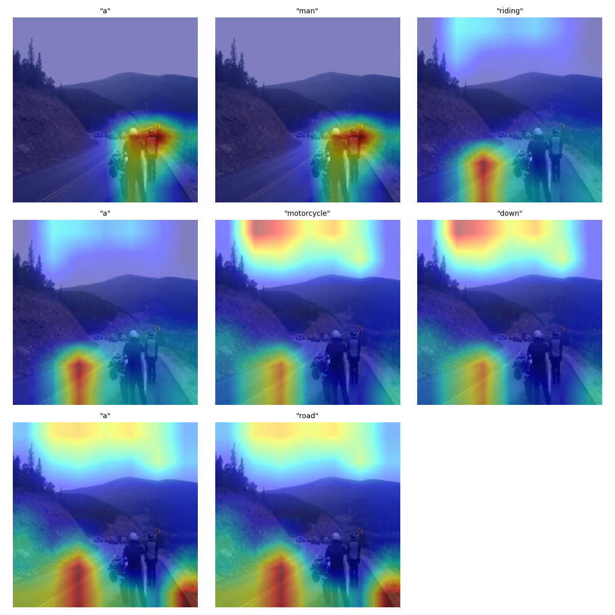
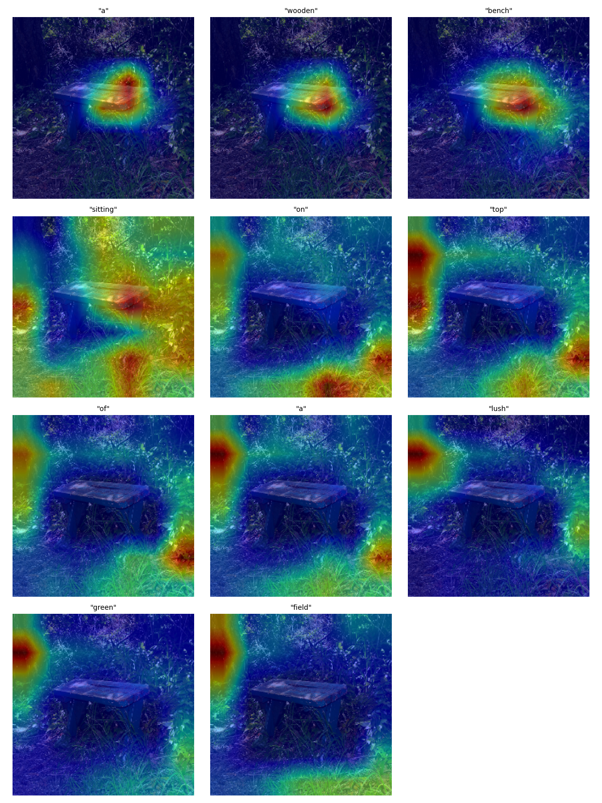
Tip: This model with beam search works much better than with the greedy strategy. When using greedy decoding, the model often repeats the same word several times in a row, frequently predicting sequences like “a a a…”. Beam search helps avoid this by exploring multiple possible continuations at each step instead of always choosing the single most probable next word — resulting in more diverse and coherent captions.
We obtain the following metrics:
| Decoding Strategy | BLEU-4 Score | CIDEr Score |
|---|---|---|
| Greedy | 0.19 | 0.628 |
| Beam Search | 0.228 | 0.698 |
Pros
- Sees image details — attention allows the model to focus on different parts of the image when generating each word.
- Produces more accurate and meaningful captions compared to Show & Tell.
- Interpretable — you can visualize where the model “looks” while generating each word.
Cons
- Slower and more complex to train and run due to attention computations at each step.
- Can get stuck on certain objects if the attention weights are not well trained.
- Still limited by the LSTM decoder — struggles with long-term dependencies and broader context.
- Unstable during inference — without a good beam search, it may repeat words or lose coherence.
Tip: You can try this implementation yourself — full code is available here.
More Attention: ViT + Transformer Decoder
As we’ve seen from previous examples, attention helps models focus better on details and generate more accurate descriptions. That’s why in the next model, ViT + Transformer, attention becomes a core part of the architecture.
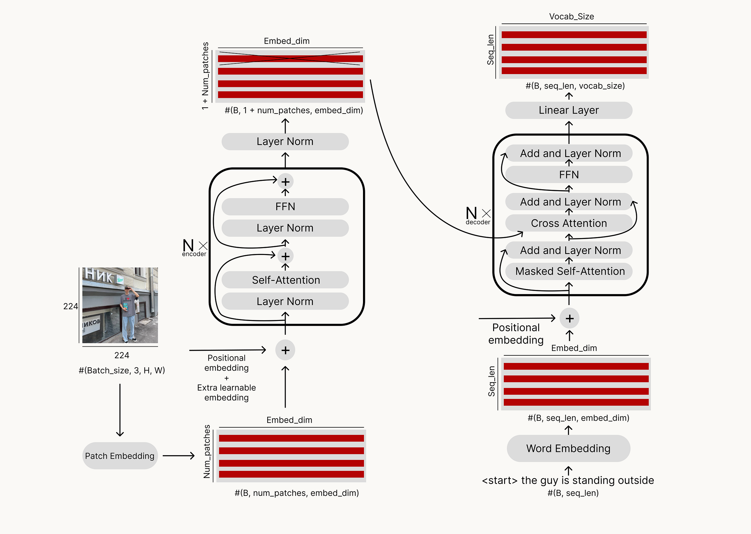
You can read more about how the Visual Transformer (ViT) works in my article I Built a Vision Transformer from Scratch — and Taught It to Pay Attention, but for now, we’ll focus on what happens after it.
Main idea: Architecture: ViT obtains the visual context, and the Transformer decoder generates captions by attending to both this visual context and its own previous predictions.
Key steps:
- ViT extracts features from the image.
- The Transformer decoder receives these features along with the previous predicted words to generate the next word in the sequence.
In the Transformer decoder, there are three key components to pay attention to: position encoding, masked self-attention, and cross-attention. Let’s go through them one by one.
Position Encoding
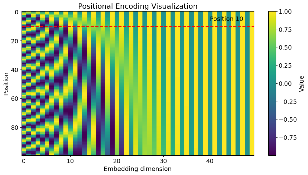
Transformers do not use recurrent or convolutional layers, so they cannot inherently detect the order of words in a sentence. To provide the model with information about the position of tokens, each word is augmented with positional encoding.
Each word receives a unique vector, where even dimensions use sine and odd dimensions use cosine, alternating across the embedding. The sines and cosines have different frequencies at different positions. This makes the position of each word unique and allows the model to distinguish between words that are close together. The dot product measures the alignment and similarity of these vectors.
If token j comes after token i, the angle between their vectors differs, and through training, the model learns to assign more or less attention depending on their relative positions.
Masked Self-Attention
You can read more about how Self-Attention works in my article on the ViT. Right now, we will understand why Masked Self-Attention is used here specifically.
The mask (usually called a causal mask or look-ahead mask) prevents the model from “looking into the future” when computing self-attention. During training, the model receives the whole sequence at once, so to prevent it from “cheating,” we limit its ability to see future tokens by effectively zeroing out (or masking) those positions in the attention calculation.
| I | love | deep | learning | <pad> | <pad> | |
|---|---|---|---|---|---|---|
| I | 1 | -∞ | -∞ | -∞ | -∞ | -∞ |
| love | 1 | 1 | -∞ | -∞ | -∞ | -∞ |
| deep | 1 | 1 | 1 | -∞ | -∞ | -∞ |
| learning | 1 | 1 | 1 | 1 | -∞ | -∞ |
| <pad> | -∞ | -∞ | -∞ | -∞ | -∞ | -∞ |
| <pad> | -∞ | -∞ | -∞ | -∞ | -∞ | -∞ |
The values of the attention matrix are multiplied by this mask before the SoftMax so that the masked positions do not affect the scores.
Tip: I also added -∞ to this mask for padding tokens, so that the model does not pay any attention to them.
To sum up: Self-Attention in the decoder looks at the words that have already been generated (using a causal mask to prevent it from seeing the future). It builds a representation of the current sentence context.
Cross-Attention
Cross-Attention is probably one of the most important parts of this architecture, as it helps the model focus on the right parts of the image. Let’s take a closer look at how it works.
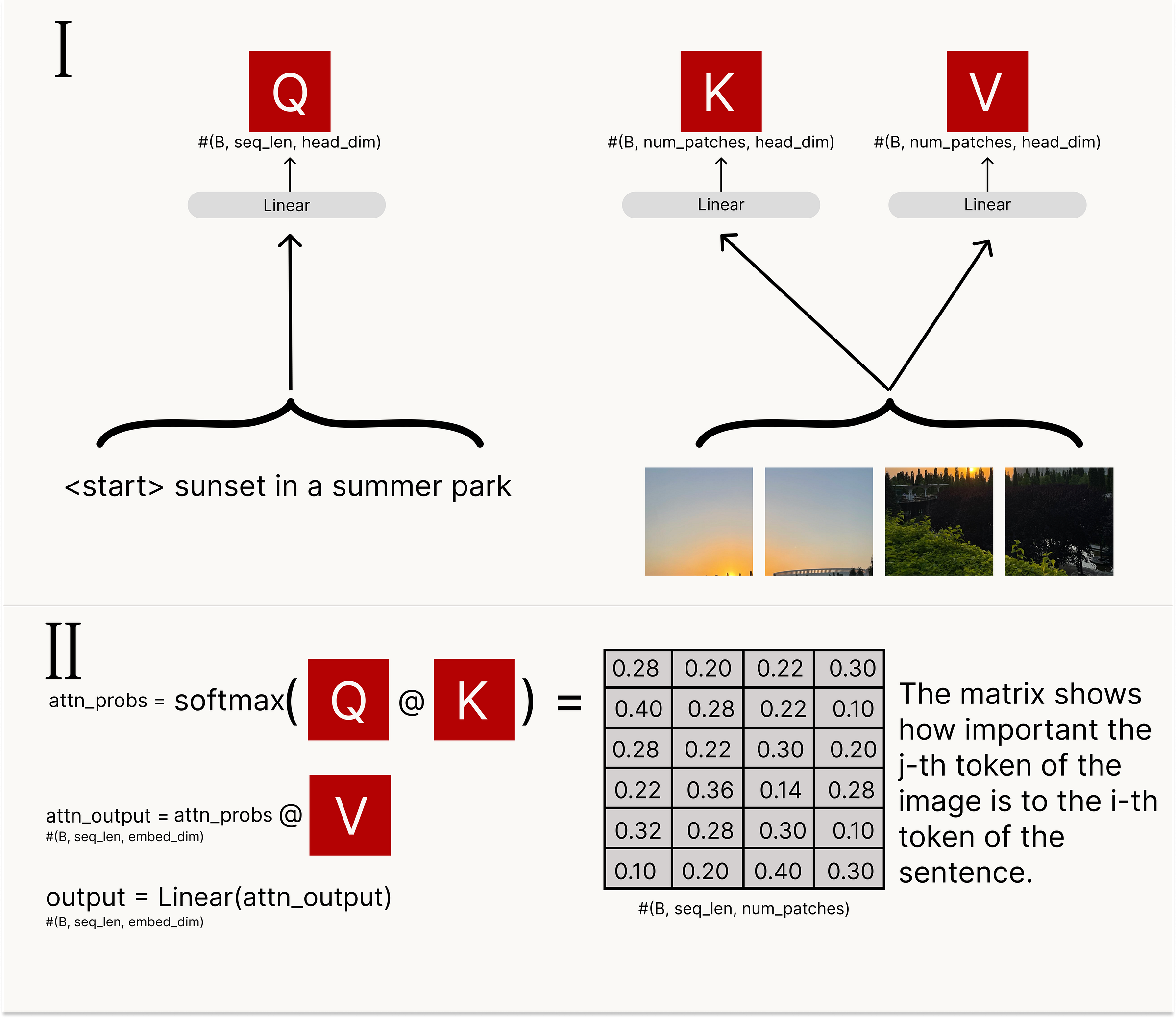
Cross-Attention takes this context and “looks” at the encoder’s output (that is — at the image). Query (Q) — are the vectors from the decoder (the current text context). Key (K) and Value (V) — come from the encoder (image patches from the ViT).
Cross-Attention determines which visual parts of the image the model should focus on to decide what makes sense to say next.
Add & LayerNorm
These are residual and layer normalization layers, used to combine the results with the original context and stabilize training through normalization.
I used the Pre-LayerNorm implementation. This provides more stable training for deep transformers (fewer gradient issues).
x = x + self.attn(self.norm1(x))
# normalization first, then the residual connection.
Feed-Forward Network (FFN)
The Feed-Forward Network (FFN) in a transformer processes each token individually after attention, enhancing and transforming the information obtained.
It adds nonlinearity and increases the model’s capacity, enabling it to create complex relationships between features.
Without the FFN, the model would be limited to linear combinations of attention and wouldn’t be able to effectively generate new words or connect text with visual features.
How they work together
- Self-Attention (causal) first looks at the words that have already been generated. It captures dependencies between them while respecting the sequence order (thanks to the causal mask). This gives a context-aware representation of the current sentence.
- Add & LayerNorm (residual 1) merges this representation with the original input, ensuring stability and preventing the model from drifting during training.
- Cross-Attention then takes this text context and “looks” at the encoder output (the image). It figures out which parts of the image are relevant for generating the next word.
- Add & LayerNorm (residual 2) again combines this cross-attended information with the previous context to keep the flow consistent and stable.
- Feed-Forward Network (FFN) processes each token individually, applying nonlinear transformations that enrich the features and allow the model to capture more complex patterns.
- Add & LayerNorm (residual 3) merges the FFN output with the prior context to stabilize learning.
- Linear + Softmax (projection) converts the final token representations into probabilities over the vocabulary, allowing the model to pick the most likely next word.
Training: During training, the model receives an image and a complete sentence that begins with a start token. Because of the mask, the model can only use the preceding words, which helps it learn to generate text correctly.
Prediction: During prediction, the model receives an image and a start token, then generates the next word. It then takes all previously generated words as input and predicts the following one, continuing this process until it produces the end token.
I trained the model with the following parameters:
- Learning rate (3e-4)
- Embedding dimension (768) — matches the hidden size of
vit-base, ensuring compatibility between the encoder and decoder. - Number of heads (12)
- Depth (6) — decoder has 6 Transformer layers.
- MLP dimension (3072)
- Dropout (0.1)
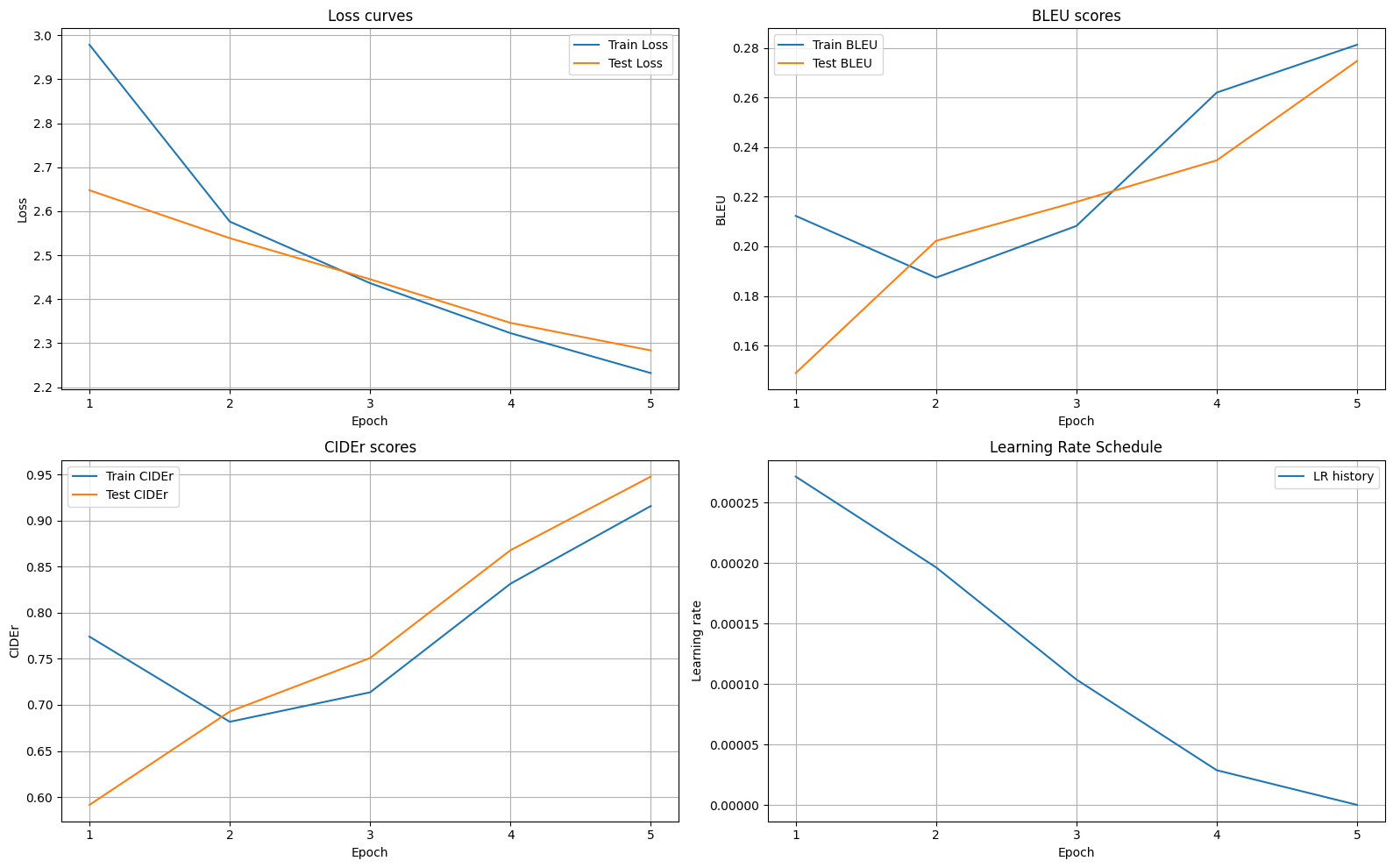
Let’s take a look at some examples of captions generated by the model:

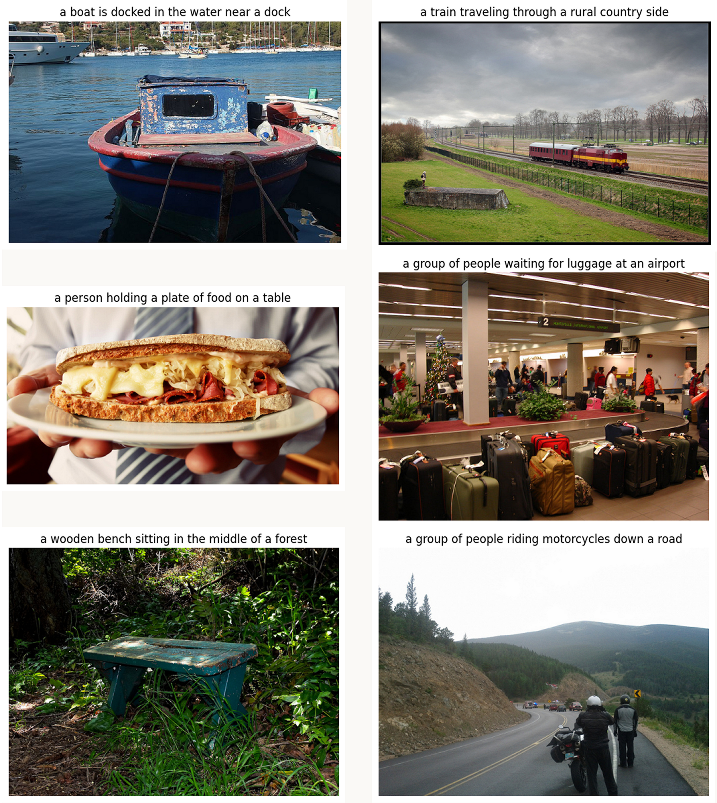
We obtain the following metrics:
| Decoding Strategy | BLEU-4 Score | CIDEr Score |
|---|---|---|
| Greedy | 0.22 | 0.74 |
| Beam Search | 0.26 | 0.80 |
Pros
- Strong feature extraction (ViT):
The Vision Transformer captures global image context through self-attention, often outperforming CNNs on large-scale datasets. - End-to-end learning:
The entire model (image encoder + text decoder) can be trained jointly, aligning visual and linguistic representations effectively. - Scalable architecture:
Both ViT and Transformer components scale well — larger versions can improve performance with more data.
Cons
- Data hunger:
Transformers (especially ViTs) require large datasets or heavy pretraining to avoid overfitting. - Computational cost:
Both ViT and Transformer decoders are memory- and compute-intensive, particularly for high-resolution images and long captions. - Slower inference:
The autoregressive decoding process generates one token at a time, making caption generation relatively slow compared to parallel methods. - Sensitivity to hyperparameters:
Training stability depends on proper learning rate schedules, warmup steps, and regularization. - Weak local feature capture (in ViT):
Without convolutional priors, ViTs may struggle to recognize fine-grained details unless trained on diverse or large-scale data. - Cross-modal alignment complexity:
The model must learn to align visual and textual representations from scratch (unless additional pretraining like CLIP is used).
Tip: You can try this implementation yourself — full code is available here.
Results at a glance
The table collects the beam-search results reported above. Higher scores are better. These are sampled validation results, not full-test-set benchmark scores; the training data differs as shown in Dataset and Evaluation.
| Model | BLEU-4, Beam | CIDEr, Beam |
|---|---|---|
| Show & Tell | 0.198 | 0.616 |
| Show Attend and Tell | 0.228 | 0.698 |
| ViT + Transformer Decoder | 0.260 | 0.800 |
From Pixels to Words
We’ve come a long way — from the first CNN+LSTM models, which saw an image as a single vector, to attention-based architectures that learned to focus on objects, and finally to modern transformers that understand the full visual and textual context.
Each generation has brought us closer to an amazing goal: machines that not only see, but also understand what they are seeing.
Today, ViT + Transformer decoders can already generate captions that are almost “human-like,” while multimodal models like CLIP and GPT combine vision and language, enabling AI to truly comprehend the world around it.
If you want to dive deeper, try implementing one of these models yourself. Start with Show & Tell, visualize attention maps in Show Attend and Tell, and experiment with a Transformer decoder built on top of a ViT. This way, you’ll not only see how everything works, but also feel how fast this field is evolving.