Vision Transformer (ViT) is an architecture that literally revolutionized how machines “see” the world.
In this article, I will not just explain what ViT is — I will show you how to build this magic yourself, step by step, even if you have never worked with transformers for image tasks before.
To begin, let’s take a look at the architecture of the Vision Transformer:
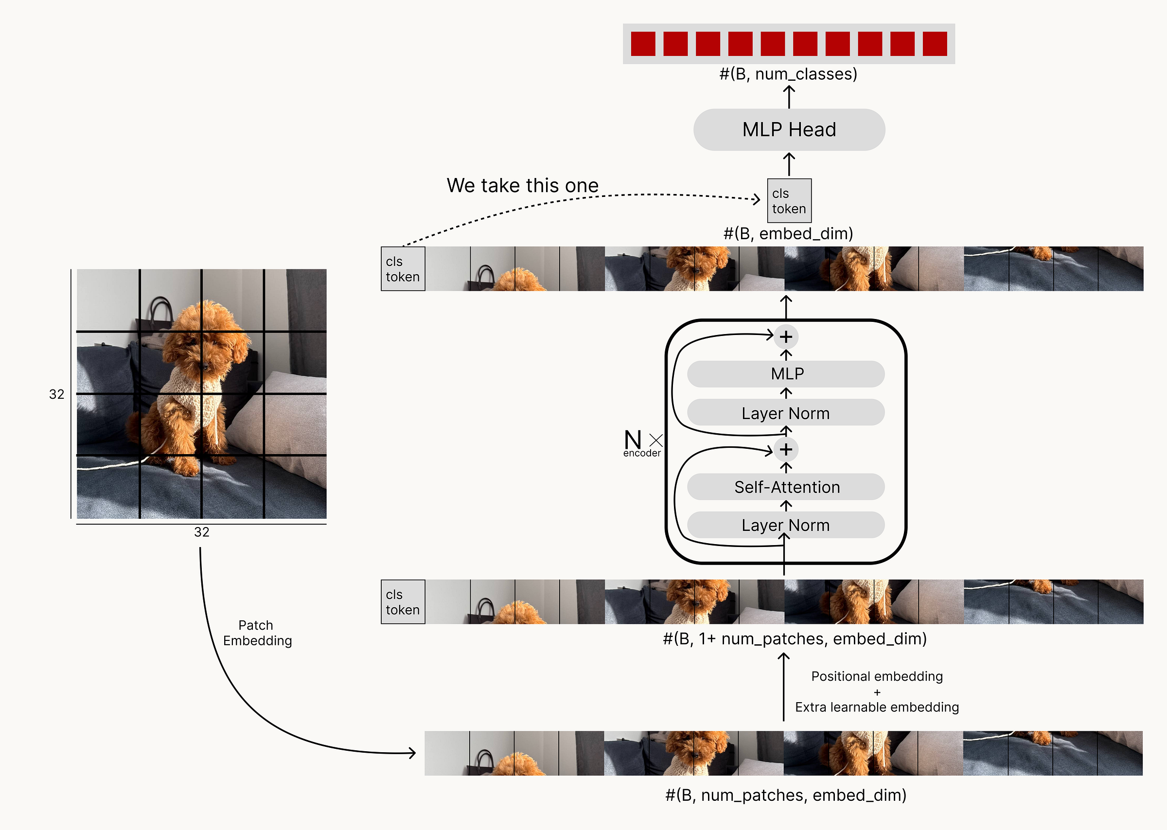
We will write the code entirely from scratch and then train the model on the CIFAR-10 dataset.
Let’s start by implementing Patch Embedding:
class PatchEmbedding(nn.Module):
    def __init__(self, img_size = 32, patch_size = 4, in_channels = 3, embed_dim=256):
        super().__init__()

        assert img_size % patch_size == 0, "img_size must be divisible by patch_size"
        self.patch_size = patch_size
        self.num_patches = (img_size//patch_size)**2
        self.conv = nn.Conv2d(in_channels, embed_dim, kernel_size=patch_size, stride=patch_size)

    def forward(self, x):
        x = self.conv(x) #(B, embed_dim, H/patch_size, W/patch_size)
        x = x.flatten(2).transpose(1, 2) #(B, num_patches, embed_dim)
        return x
The image will be divided into patches, and the size of each patch can be specified using the patch_size parameter. The image is not only divided into patches but also passed through CNN kernels. As a result, we don’t just get image patches — we get embeddings of those patches.
The next step is to implement the most interesting part of this model — the attention mechanism.
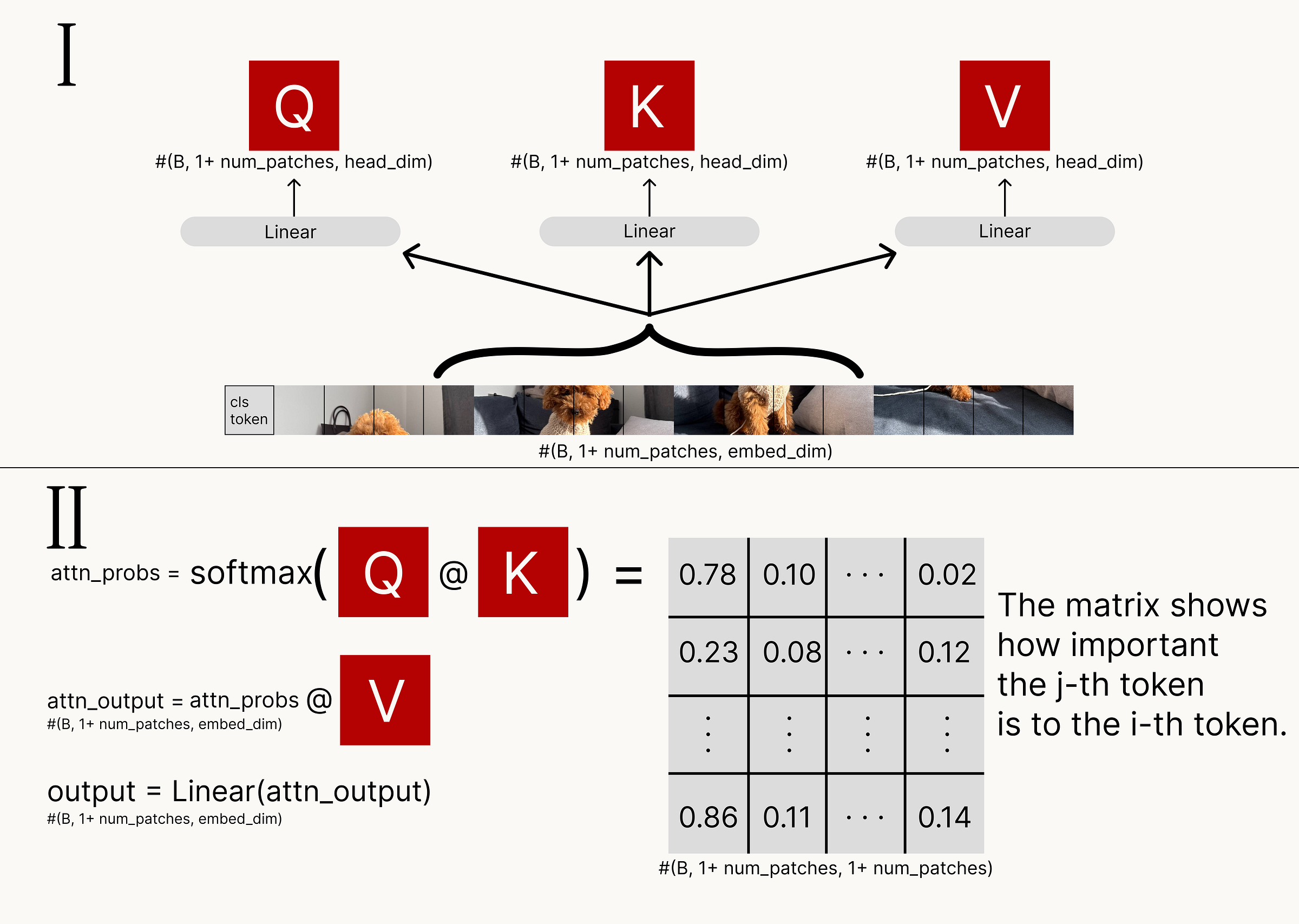
Q (Query) formally poses a question from each patch to the other patches, K (Key) indicates whether each patch has an answer to that question, and V (Value) contains the “values,” the actual data of each patch that will be used to form the final representation.
Suppose we have X and Y, and we want X to pay attention to Y. In that case, the Query matrix is multiplied by X, while the Key and Value matrices are multiplied by Y. Instead of multiplying by matrices, we use linear layers.
attn_probs are the attention matrices that show how much token i should "attend to" token j. Next, we multiply this by V to obtain the image embeddings based on attn_probs. V essentially stores the values of each image patch, while attn_probs shows how much each patch should take from every other patch.
This is how one attention head works; then the values from all heads are combined. They are designed with the idea that each head focuses on something different.
class MultiHeadAttention(nn.Module):
    def __init__(self, dim, num_heads, dropout):
        super().__init__()
        assert dim % num_heads == 0, "Embedding dimension must be divisible by number of heads"
        self.num_heads = num_heads

        self.head_dim = dim // num_heads

        self.qkv = nn.Linear(dim, dim * 3, bias = False)
        self.out = nn.Linear(dim, dim, bias = False)

        self.scale = 1.0 / (self.head_dim ** 0.5)

        self.attn_dropout = nn.Dropout(dropout)

    def forward(self,  x, mask = None,  return_attn=False):
        B, num_patches, embed_dim = x.shape

        qkv = self.qkv(x) # (B, num_patches, 3*embed_dim)
        qkv = qkv.reshape(B, num_patches, 3, self.num_heads, self.head_dim)
        qkv = qkv.permute(2, 0, 3, 1, 4) #(3, B, num_heads, num_patches, head_dim)

        q, k, v = qkv[0], qkv[1], qkv[2]  # each (B, num_heads, num_patches, head_dim)

                                        #How important it is for token i to pay attention to token j.
        attn_scores = (q @ k.transpose(-2, -1)) * self.scale #[B, num_heads, N, N]

        if mask is not None:
            # mask: (B, 1, N, N) or (1, 1, N, N)
            attn_scores = attn_scores.masked_fill(mask == 0, float("-inf"))

        attn_probs = attn_scores.softmax(dim=-1) #[B, num_heads, N, N]
        attn_probs = self.attn_dropout(attn_probs)
        attn_output = attn_probs @ v  # (B, num_heads, num_patches, head_dim)
        attn_output = attn_output.transpose(1, 2).reshape(B, num_patches, embed_dim)

        if return_attn:
          return self.out(attn_output), attn_probs
        else:
          return self.out(attn_output) #(B, num_patches, embed_dim)
Let’s proceed with assembling the Transformer Encoder block:
class TransformerEncoderBlock(nn.Module):
    def __init__(self, dim, num_heads, mlp_dim, dropout):
        super().__init__()
        self.norm1 = nn.LayerNorm(dim)
        self.attn = MultiHeadAttention(dim, num_heads, dropout)
        self.norm2 = nn.LayerNorm(dim)

        self.mlp = nn.Sequential(
            nn.Linear(dim, mlp_dim),
            nn.GELU(),
            nn.Dropout(dropout),
            nn.Linear(mlp_dim, dim),
            nn.Dropout(dropout)
        )
        self.dropout = nn.Dropout(dropout)

    def forward(self, x, return_attn=False):
      if return_attn:
        attn_out, attn_weights = self.attn(self.norm1(x), return_attn=True)
        x = x + self.dropout(attn_out)
        x = x + self.dropout(self.mlp(self.norm2(x)))
        return x, attn_weights
      else:
        x = x + self.dropout(self.attn(self.norm1(x)))
        x = x + self.dropout(self.mlp(self.norm2(x)))
        return x
Here, we are simply following the architecture of our network — we’ve already implemented all the necessary blocks.
We’re already nearing the end — now we’ll be assembling the Vision Transformer itself:
class VisualTransformer(nn.Module):
    def __init__(self,num_classes, img_size=32, patch_size=4, in_channels=3, embed_dim=256,
                 num_layers=6, num_heads=7, mlp_dim=512, dropout=0.1):
        super().__init__()

        self.patch_embed = PatchEmbedding(img_size, patch_size, in_channels, embed_dim)
        self.cls_token = nn.Parameter(torch.randn(1, 1, embed_dim))
        self.pos_embed = nn.Parameter(torch.randn(1, 1 + self.patch_embed.num_patches, embed_dim))
        self.dropout = nn.Dropout(dropout)

        self.encoder_blocks = nn.ModuleList([
                TransformerEncoderBlock(embed_dim, num_heads, mlp_dim, dropout)
                for _ in range(num_layers)
            ])

        self.norm = nn.LayerNorm(embed_dim)

        self.mlp_head = nn.Sequential(
            nn.LayerNorm(embed_dim),
            nn.Linear(in_features=embed_dim, out_features=num_classes)
        )

    def forward(self, x, return_attn = False):
        B = x.size(0)
        x = self.patch_embed(x)  # (B, N, D)

        cls_tokens = self.cls_token.expand(B, -1, -1)  # (B, 1, D)
        x = torch.cat((cls_tokens, x), dim=1)  # (B, 1+N, D)
        x = x + self.pos_embed
        x = self.dropout(x)

        attn_maps = []
        for block in self.encoder_blocks:
          if return_attn:
            x, attn = block(x, return_attn=True)
            attn_maps.append(attn)  # (B, heads, N, N)
          else:
            x = block(x) # (B, 1+N, D)

        x = self.norm(x)

        out = self.mlp_head(x[:, 0, :])

        if return_attn:
          return out, attn_maps
        else:
          return out
Here we need to clarify a few things. What is the cls_token? It’s a special token that we add manually, and it has the same size as the image patches. Its purpose is to be used later for image classification. The idea is that, as it passes through the Attention blocks, this token gathers information about the entire image.
Next, let’s look at pos_embed. Since we divide the image into patches and then align them in a sequence — as if we were working with text — the model has no inherent understanding of the spatial relationships between the patches. To address this, we add positional information to the patches. In our case, this pos_embed is a learnable parameter.
With the mlp_head, it’s simple: it takes the cls_token, passes it through a linear layer, and classifies our image.
After assembling our model, let’s proceed to training.
For training, we will use the following hyperparameters:
BATCH_SIZE = 128
EPOCHS = 80
LEARNING_RATE = 3e-4
PATCH_SIZE = 4
NUM_CLASSES = 10
IMAGE_SIZE = 32
CHANNELS = 3
EMBED_DIM = 256
NUM_HEADS = 8
DEPTH = 6
MLP_DIM = 512
DROP_RATE = 0.1
Let’s take a look at the number of parameters:
Total parameters: 3,189,514
Trained parameters: 3,189,514
And the following augmentations:
train_transforms = transforms.Compose([
    transforms.Resize((70, 70)),
    transforms.RandomResizedCrop(32, scale=(0.8, 1.0)),
    transforms.RandomHorizontalFlip(p=0.5),
    transforms.RandomRotation(15),
    transforms.ColorJitter(0.2, 0.2, 0.2, 0.1),
    transforms.RandomAffine(degrees=0, translate=(0.1, 0.1), scale=(0.9, 1.1)),
    transforms.ToTensor(),
    transforms.Normalize((0.5, 0.5, 0.5), (0.5, 0.5, 0.5)),
    transforms.RandomErasing(p=0.25, scale=(0.02, 0.2), ratio=(0.3, 3.3), value='random'),
])
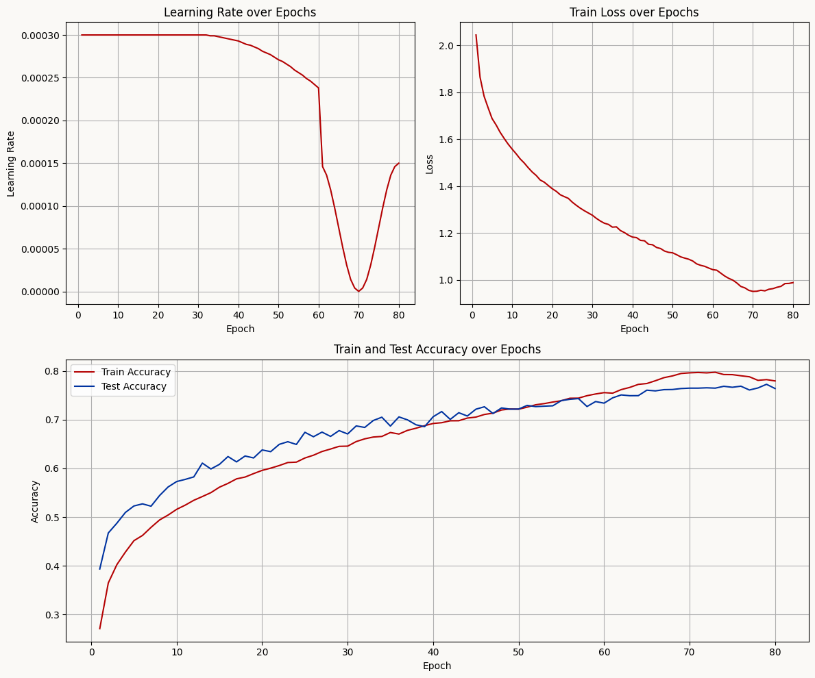
We train the model and obtain the following results:
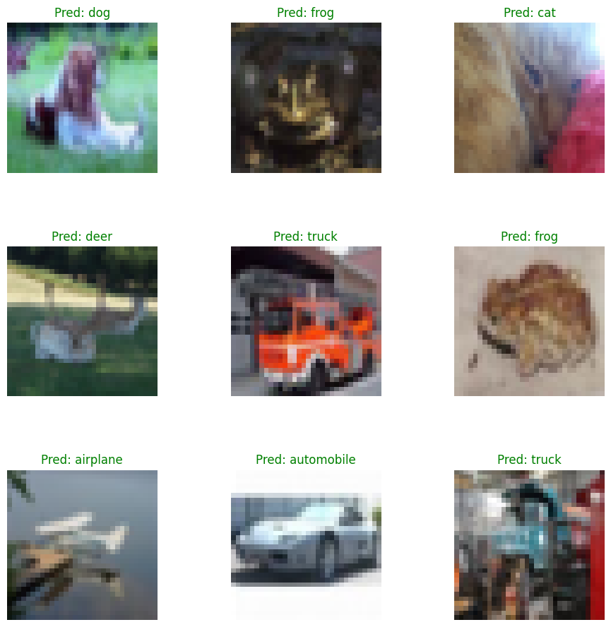
Let’s take a look at the model’s predictions:
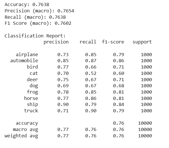
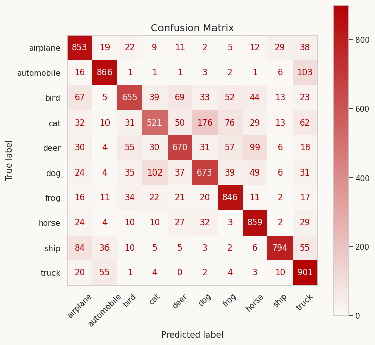
Here are the metrics of the resulting model:
Now for the most interesting part — attention. Let’s see what our model focuses on during classification:
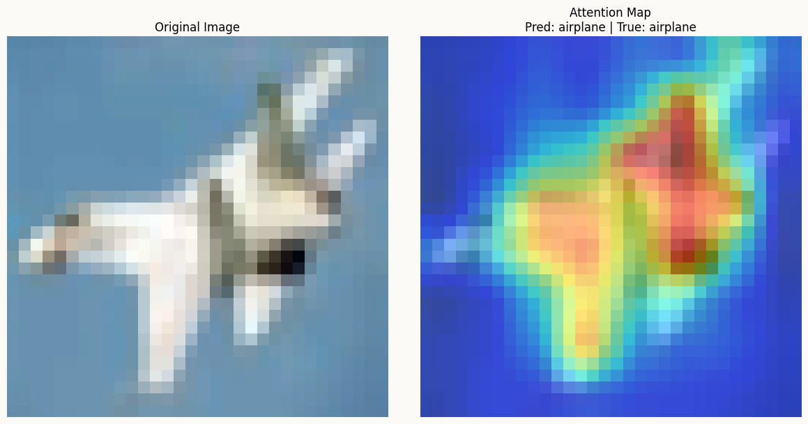
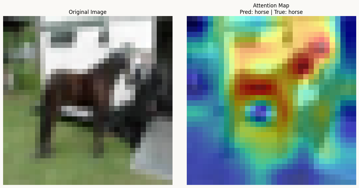
In this article, we walked through the implementation of the Vision Transformer and its attention mechanism. We looked at what this model is capable of and how it “looks” at an image using the attention mechanism. The Vision Transformer has opened new directions in computer vision research by combining ideas from NLP and image processing. In the future, we will definitely apply this model to Image Captioning.
You can find the complete code and training process on my Kaggle:
https://www.kaggle.com/code/nickr0ot/visual-transformer-from-scratch